Introduction
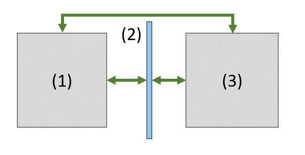
Area Junctions are special in SEA theory. For cavity-plate-cavity connections there are not only direct paths. This violates the principle SEA assumption that only connected subsystems can exchange energy
An intrusive way to understand the different paths is the transmission formula from Cremer.
\tau(\vartheta) = \left[ \left( \frac{m''\omega}{\rho_0c_0}\right)^2 \{\frac{k_a^4\sin^4\vartheta}{k_B^4}-1\}^2 \cos^2\vartheta+1\right]^{-1} and
and  are mass per area, fluid density and speed of sound, respectively.
  and
and  are the cavity air and plate bending wavenumber.
  is the angle of the incoming wave to the plate normal.
The  term represents the two paths going through the bending wave field of the plate. As this are the paths that connect the wave field of the plate with the reverberant field of the cavity those paths are called the resonant paths. The plate resonates and retains energy.
The  correspond to the direct path connection between both cavities. Better known as mass law and called the non-resonant path in the SEA theory. The plate experiences a forced motion and no energy is retained in the plate
Resonant Coupling Loss Factor
How is the resonant coupling loss factor (CLF) calculated? It is common practice to apply the radiation efficiency  .
.
\eta_{21} = \frac{\rho_0c_0}{m''\omega}\sigmaThe formula is simple – the devil is in the calculation of the radiation efficiency, which is not that easy. Details are given in section 8.2.3.4 of my book.
Non-resonant Couling Loss Factor
The non-resonant coupling loss factor is calculated from the mass-law transmission coefficient  . CLF and transmission coefficient are related for 2D couplings by:
\eta_{13} = \frac{k_a^2 S_j\tau_{mass}}{8\pi^2n_1(\omega)\omega}Twin chamber example
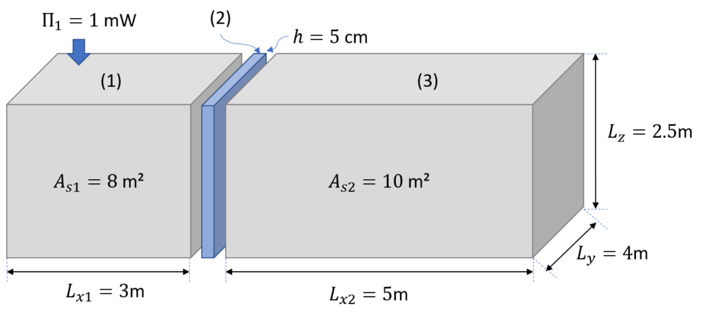
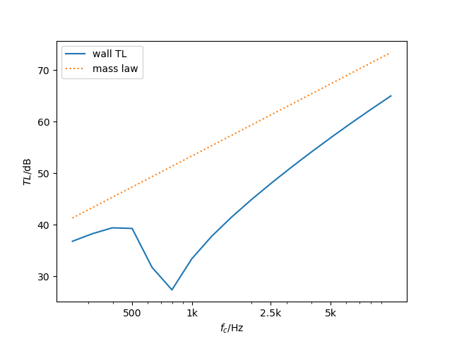
The example is described in detail in the pyva documentation. The result is the TL of the wall is shown as follows. You may guess which kind of material and wall we have here…
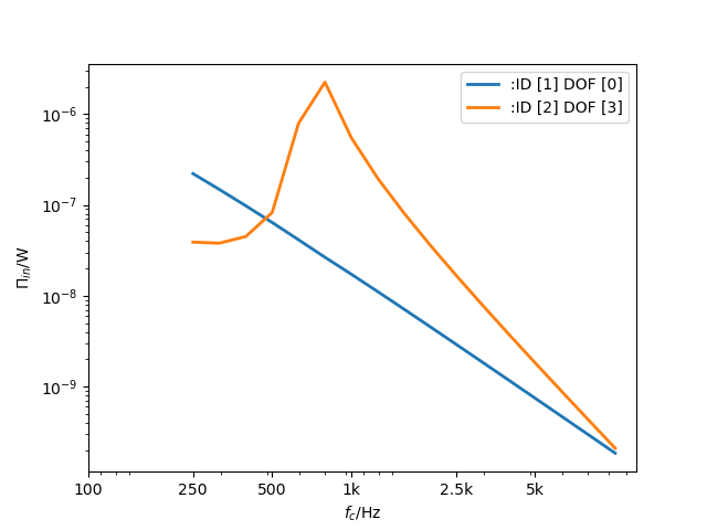
One big advantage of SEA is, that contribution of each path can be monitored in detail. The following figure shows why concrete walls are not always a good idea (especially when very thin) in modern Buildings. The excellent radiation efficiency of the concrete wall transmits the acoustic power too well.