Modelling Sound Transmission through Double Panels Using Pyva

The paper from Price and Crocker¹ more than fifty years ago initiated a still ongoing discussion about modelling double panel sound transmission using statistical energy analysis. This sometimes confusing discussion results from the fact, that the double wall case establishes a very critical case for SEA for several reasons that will be elaborated here in detail. This is done using the pyva toolbox applied to the examples from Price’ original paper.

A step by step description summarizes the modelling of the examples from the original paper revealing the power of SEA modelling of double walls but also showing the limits of SEA when the basic prerequisites are not met. Each single figure and example case is shown as pyva implementation comparing the results from the original paper.

Library initialization and model setup

In the paper several double wall configurations are modeled using SEA. The theory is implemented in pyva and the major steps of this modelling are shown here. If you are interested in following the examples please refer to the pyva documentation where the full example can be downloaded.

Module import

Each pyva simulation script starts with the import of the related modules

# pyva main model module 
import pyva.models as mds

# Coupling module
import pyva.coupling.junctions as con    # junctions module

# Property modules
import pyva.properties.structuralPropertyClasses as stPC
import pyva.properties.materialClasses as matC

# Layer module for transfermatrix methods
import pyva.systems.infiniteLayers as iL

# SEA system modules
import pyva.systems.structure2Dsystems as st2Dsys # plate systems module
import pyva.systems.acoustic3Dsystems as ac3Dsys  # cavity systems moduke 
import pyva.loads.loadCase as lC                  # loadcase module

# Modules for system matrices and degree of freedom
import pyva.data.dof as dof
import pyva.data.matrixClasses as mC

# Pyva utilities
import pyva.useful as uf

Initialization of geometry

Frequency range and geometry are initialized using python variables. The double cavity is well defined but the properties of the main cavities are not specified in detail. For simple transmission loss calculations cavities (1) and (5) are chosen as large cavities to fulfill the random conditions and the absorption surface $A_s$ in the receiving cavity is equal to the junction area $A_s=S_j$ . This simplifies the transmission loss calculation because in

TL = L_p^{(1)}-L_p^{(5)} -10 \log_{10}\frac{S_j}{A_s}\overset{S_j=A_s}{=}L_p^{(1)}-L_p^{(5)}

and $10\log_{10}S_j/A=0$ the transmission loss is simply the difference of the pressure levels.

#%% Frequency range
omega = mC.DataAxis.octave_band(f_min=2*np.pi*100,f_max=2*np.pi*10000,bands_per_octave = 3)
# Create according ndarrays for plotting
om    = omega.data
freq  = om/2/np.pi 

# Panel dimensions
L1 = 1.55   # panel/DW cavity width
L2 = 0.071  # DW cavity thickness
L3 = 1.97   # panel/DW cavity height

L1_fig3 = 2.2 # height of cavity from fig 3

S = L1*L3   # panel surface
S_dwc_edge = L2*2*(L1+L3)# DW cavity edge surface

# Cavity volumes
V_dwc  = L1*L2*L3 # Volume DW cavity
V1 = 100 # room 1
V2 = 100 # room 2

# Absorption areas in large cavities
As1  = 2. # arbitrary room absorption area
As2  = S  # secong room absorption area equal to junction area for log10(S/As2)=0

Material and Properties

In the paper all plates are aluminum panels of various thicknesses that are used in further calculations. The Fluid and IsoMat Classes of the materialClasses module are used. The plate thickness is specified using the PlateProp of the structuralProperty module.

# Materials
alu = matC.IsoMat(eta=0) # Alu is the default isomaterial
air = matC.Fluid(eta=0)  # Air is the default fluid

# Plate properties
alu_3_18mm = stPC.PlateProp(0.00318,alu) # 0.85 g/cm^2
alu_6_36mm = stPC.PlateProp(0.00636,alu) # 1.71 g/cm^2
alu_0_88mm = stPC.PlateProp(0.00088,alu) # 0.24 g/cm^2
alu_9_26mm = stPC.PlateProp(0.00925,alu) # 2.5  g/cm^2

Subsystem definition

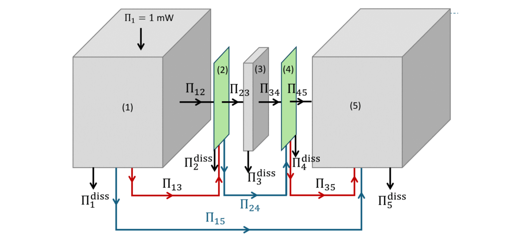
There are two type of subsystems involved. Flat rectangular plates and cavities. All SEA system classes are located in the systems package. This package provides classes and methods to deal with the properties of SEA subsystems and conversion of energy results into engineering units. Each subsystem is identified by an integer ID as first argument following the numbering convention of the paper.

Cavities

Cavities are created using Acoustic3DSystem module. The large sending and receiving room are supposed to be artificial cavities with volume but without surface and perimeter. This means that only the volume is used for the modal density determination in Equation #maa-equation.

# Cavity subsystems
room1 = ac3Dsys.Acoustic3DSystem(1, V1, 0, 0, air, absorption_area = As1, damping_type= ['surface'])
room2 = ac3Dsys.Acoustic3DSystem(5, V2, 0, 0, air, absorption_area = As2, damping_type= ['surface'])

The double wall cavity is rectangular. Therefore, the RectangularRoom class is used that implements methods (and assumptions) specifically true for this kind of cavity. Price assumed that the radiation efficiency doubles below the coincidence frequency because of the flat cavity. This is now implemented in pyva, the flat_cavity_sw triggers this doubled radiation efficiency.

# Double wall cavity
dwc     = ac3Dsys.RectangularRoom(3, L1, L2, L3, air, eta = eta_DWC,flat_cavity_sw = True)

Damping loss factor of double wall cavity

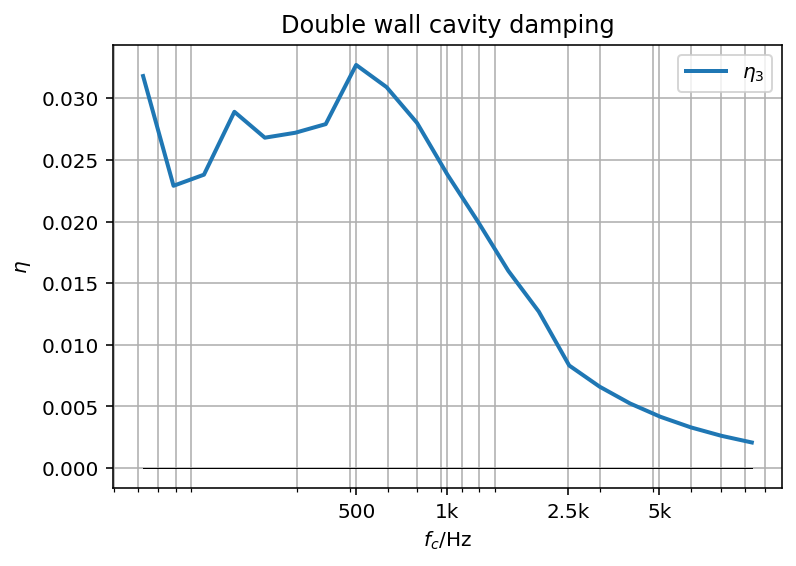
In the RectangularRoom constructure the damping is specified by the eta = eta_DWC argment. This value can be a constant but also a Signal, here a spectrum that specifies a frequency-dependent damping according to the paper. From 100-2000 Hz the damping loss is taken from table B-I of the paper. Above 2000 Hz equation (B11) is used with $\alpha_0 = 1$ .

#Tables for DW cavity damping
omega_min = 2*np.pi*100       # in all arguments pyva uses angular frequency
omega_max = 2*np.pi*10000
freq_tab_BI = mC.DataAxis.octave_band(omega_min,omega_max,typeID = 21)
 
# Create table until 10000Hz
eta_DWC_data = np.zeros(np.shape(freq_tab_BI))
# Fill data until 2000 Hz
eta_DWC_data[0,:14] = 0.01*np.array([[3.18, 2.29, 2.38, 2.89, 2.68, 
                         2.72, 2.79, 3.27, 3.09, 2.80,
                         2.38, 2.00, 1.60, 1.27 ]])

# Fill data from 3200 - 10000 Hz with equation  B11
def B11(omega):
    return air.c0*S_dwc_edge/6/omega/V_dwc     # alpha = 1

eta_DWC_data[0,14:] = B11(freq_tab_BI.data[14:])

# Signal object with scalar degree of freedom and unit-less type 
eta_DWC = mC.Signal(freq_tab_BI, eta_DWC_data, dof.DOF(0,0,dof.DOFtype(typeID = 1)))

The python codes creates the damping spectrum as shown in the following figure:

**Fig.**: Damping loss according to Table B-I and Equation (B11)

Plates

Plate subsystem are created using the RectangularPlate class from the structural2Dsystem module. The convention is that all plates are named in relation to the figure in Price paper the results are presented, here figure 5.

# Plate subsystems
plate1_fig_5 = st2Dsys.RectangularPlate(2, L1,L3,prop=alu_3_18mm, eta = 0.005) 
plate2_fig_5 = st2Dsys.RectangularPlate(4, L1,L3,prop=alu_3_18mm, eta = 0.005)

Double wall frequencies

It is surprising that the double wall frequency that separates the single wall from the double wall dynamics is not considered at all. For further discussions the double wall frequency is calculated by:

f_{DW}=\frac{1}{2\pi}\sqrt{\frac{\rho_0c_0^2}{L_2\mu}} \text{ with } \mu'' = \frac{m''_1m''_2}{m''_1+m''_2}

Here $\mu''$ , $m''_1$ and $m''_2$ are the effective mass per area, the first panel mass per area and the second panel mass per area, respectively. The resulting frequencies are as follows:

Double wall resonance Fig.5: 109.7Hz
Double wall resonance Fig.6: 95.0Hz
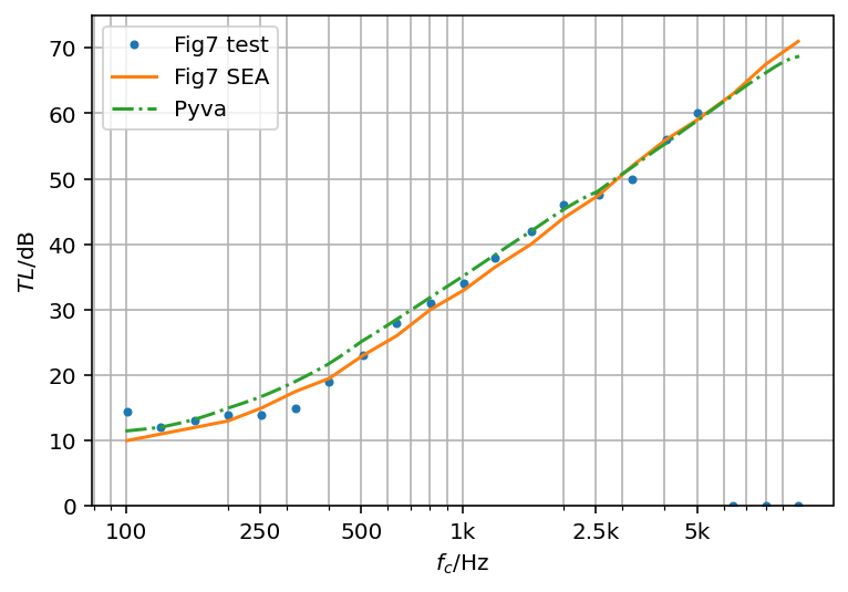
Double wall resonance Fig.7: 166.6Hz

Modal density and modes in band

Every SEA simulation starts with investigating the statistical quantities of the involved subsystems. In the paper the modal density is calculated using the formula for 2D cavities (Eq.(28)) and 3D cavities (Eq. (29)). Both regimes are separated by the cross-mode frequency $f_d=\frac{c_0}{2L_2}$ . In Figure 3 the results from the classical Maa² formula and the paper results are compared to the numerical result counting the modes in the double wall cavity.

The Maa formula used in all commercial SEA software and also pyva is given by:

n(\omega)=\frac{V\omega^2}{2\pi^2c_0^3}+\frac{S\omega}{2\pi^2c_0^2}+\frac{P}{16\pi c_0}

With the volume $V$ , the surface $S$ and the perimeter $P$ .

The formula from Price performs best, the thin cavity establishes a clear distinction between the two- and three dimensional case. Note that the dimensions of Fig.3 are not the same as for the double wall cavity of all other calculations.

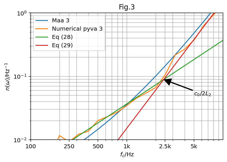
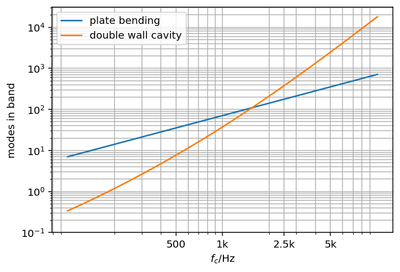
Fig.3: Modal density of the (modified) double wall cavitiy using variopus models — **Fig.3:** Modal density of the (modified) double wall cavity

However, the modal density below 500 is very low. Too low for this even larger cavity to be considered as random system. When the number of modes counted per octave band is calculated it can be seen that a reasonable number of modes is reached starting from the 500Hz third octave. Thus, the double wall cavity cannot be considered as random subsystem below 500 Hz.

Modes in band of plate and double wall cavity — Fig. 4: Modes in third octave band of plate and double wall cavity.

SEA model creation

Each model required a defined analysis frequency range. The DataAxis class of the matricClasses does this job.

omega = mC.DataAxis.octave_band(f_min=2*np.pi*100,f_max=2*np.pi*10000,bands_per_octave = 3)

The SEA model is defined using the HybridModel class. This class combined FEM and SEA system descriptions. In our case only the SEA part is used.

SEA_model = mds.HybridModel((room1,plate1_fig_5,dwc,plate2_fig_5,room2),xdata=omega)

The connection of the subsystem is defined by junctions, here shown for the example of Fig.5

#%% Junctions Fig 5 Model
J123_fig_5 = con.AreaJunction((room1,plate1_fig_5,dwc))
J345_fig_5 = con.AreaJunction((dwc,plate2_fig_5,room2))

Those junctions must be added to the SEA model:

SEA_model.add_junction({'areaJ_123':J123_fig_5})
SEA_model.add_junction({'areaJ_345':J345_fig_5})

The model is now complete, except the sound source in room1

# Source in cavity 1
power1mWatt = lC.Load(omega, 0.001*np.ones(omega.shape), 
                      dof.DOF(1,0,dof.DOFtype(typestr = 'power')), name = '1mWatt')
SEA_model.add_load('1mWatt',power1mWatt)

Solving the model

The remaining job is to setup the SEA matrix an solve the model:

SEA_model.create_SEA_matrix(sym = 1)
SEA_model.solve()

Pyva automatically calculated the engineering units from the energy results. Requesting the results gives:

SEA_model.result
Out[8]: 
Signal object of 21 samples with 7 channels and properties ...
DataAxis of 21 samples and type angular frequency in 1 / second
DOF object with ID [1 2 2 3 4 4 5], DOF [0 3 5 0 3 5 0] of type 
[DOFtype(typestr='pressure'), 
DOFtype(typestr='velocity'), DOFtype(typestr='velocity'), 
DOFtype(typestr='pressure'), 
DOFtype(typestr='velocity'), DOFtype(typestr='velocity'), 
DOFtype(typestr='pressure')]

All results are presented as Signals. This includes the IDs the degrees of freedom DOF an the nature of the results. Note that plates have two wave DOFs for bending waves (DOF=3) and in-plane waves (DOF=5).

The missing step is to calculate the transmission coefficient keeping in mind that the difference of the pressure levels corresponds to the ratio of the squared pressure. The room pressure results are the signals with index 0 and 6.

    p1 = SEA_model.result[0].ydata.flatten()
    p2 = SEA_model.result[6].ydata.flatten()
    tau = (p2/p1)**2

With this global procedure all examples from Price paper are recalculated.

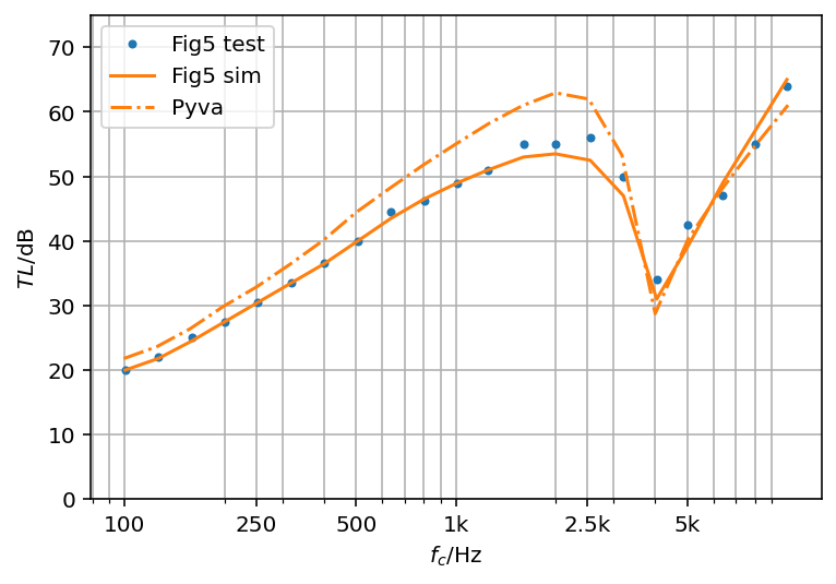
Two aluminum plates of 3.18mm thickness

The symmetric case of figure 5 is the first case in the paper. Figure 5 reveals that the pyva results are much higher below coincidence compared to the surprisingly well coinciding test and SEA results from the original paper. The double wall resonance is not visible in the test results. The curve doesn’t show the typical double panel behavior as it is for example described in Fahys book³

Figure 5 of Price SEA paper showing the paper curves and the pyva SEA result. — **Fig.5:** Transmission loss of double panel system

The reason for this discrepancy to current SEA implementations (and double wall theory) is hidden in the radiation efficiency or the radiation resistance as used by Price. The authors solve the SEA equations for bending wave excitation into plate 1. This provides the radiation resistance of the plate from test results exciting the plate at several locations. Because of this procedure every side paths that are not considered in the model are taken into account automatically and the SEA model result is adapted to the test results accidentally including the strong coupling, structure borne coupling and even additional paths.

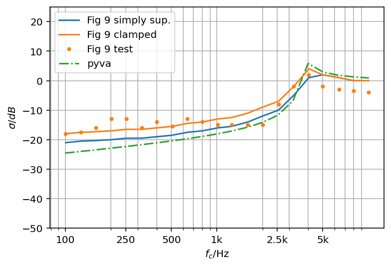
This can be seen when the radiation efficiency from pyva based on the Leppington⁴ method is compared to Figure 9 of the paper. The so called clamped result agrees well with the test result (that may include many paths). The pyva result is 10dB lower than the test. Form the authors experience from numerical studies and tests the radiation efficiency below coincidence is too high.

Fig.9: Radiation efficiency from original paper and pyva.

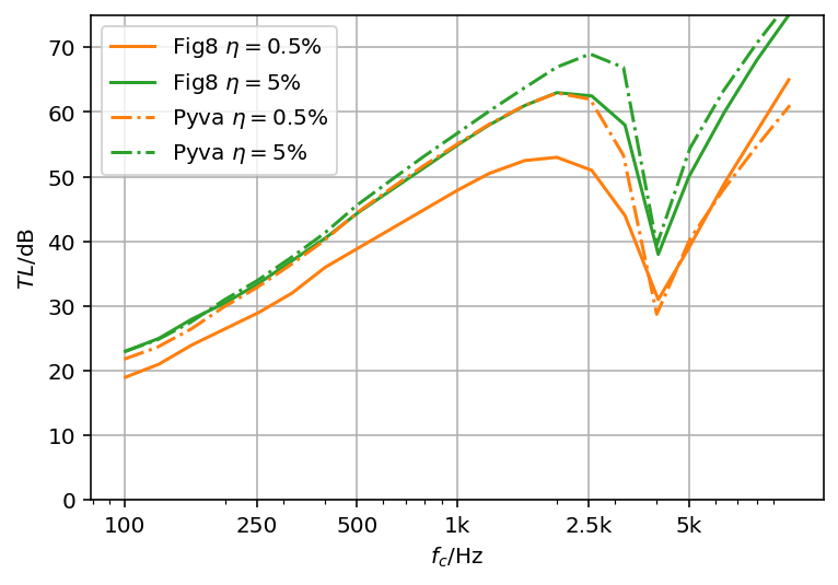
This high radiation efficiency may be the reason why the damping influence is too strong especially below coincidence. In Fig. 8 the high 5% damping loss has low impact below coincidence in the pyva results whereas the paper denotes a broadband shift that is too strong and is not in line with numerical and test results of a single plate.

**Fig.8:** Variation of transmission loss from paper and pyva simulation

Please note, that at and above coincidence when all SEA assumptions are fulfilled, paper and pyva results agree very well with the test results.

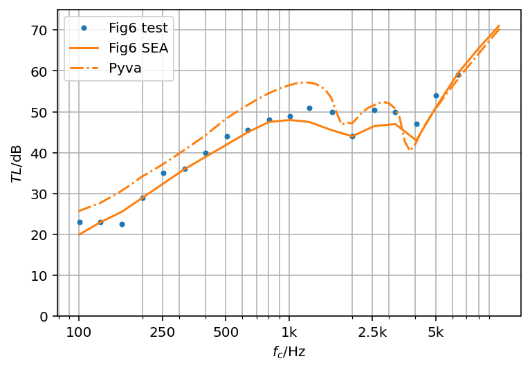
Two different aluminum plates of 6.36 mm and 3.18 mm thickness

The second example is a non-symmetric configuration with one plate doubled in thickness. The resuls from pyva and from Figure 6 in the paper show the distinct coincidence frequencies. Paper and pyva results agree well above the second coincidence but below coincidence the transmission loss is also underestimated. However, the pyva result agrees better to the tests above the first coincidence of the thicker 6.38 plate at $f_c=1870$ Hz.

**Fig.6**: Transmission loss of 6.36 and 3.18 mm double panel system

Two thin 0.88mm panels without coincidence

An interesting case is created with two aluminum panels of 0.88mm thickness. The coincidence of such panels is at $f_c=13517$ Hz and therefore above highest simulation and test frequency. The double wall resonance is at $f_{dw}=166$ Hz. With this configuration the radiation efficiency of both panels is very low and the mass law dominates. Thus, the agreement between the original paper, pyva and the tests is quite above 500 Hz when the SEA assumptions are fulfilled. A slight double wall dipp may be noticed in the test data.

**Fig.6**: Transmission loss of 0.88 mm double panel system

Variation of double wall thickness

References

J. Price, and M.J. Crocker, “Sound Transmission through Double Panels Using Statistical Energy Analysis,” J. Acoust. Soc. Am. 47, 683–693, (1970) ↩︎
D. Maa, “Distribution of Eigentones in a Rectangular Chamber at Low Frequency Range,” J. Acoust. Soc. Am. 10, 235–238, (1939) ↩︎
F. Fahy, Sound and Structural Vibration: Radiation, Transmission and Response. Academic Press, 1985 ↩︎
F. G. Leppington, E. G. Broadbent, and K. H. Heron, “The Acoustic Radiation Efficiency of Rectangular Panels,” Proc. Royal Society A: Mathematical, Physical and Engineering Sciences, 382, pp. 245–271, Aug. 1982 ↩︎